# Dr. M. Baron, Statistical Machine Learning class, STAT-427/627

# DECISION TREES

1. Classification trees

> library(tree)

Define a categorical variable ECO

> ECO = ifelse( mpg > median(mpg), "Economy", "Consuming" )

> Cars = data.frame( Auto, ECO ) # Include ECO into the data set

> table(ECO)

Consuming Economy

196 196

# Here is the main tree command.

> tree( ECO ~ .-name, Cars )

1) root 392 543.4 Consuming ( 0.5 0.5 )

2) mpg < 22.75 196 0.0 Consuming ( 1.0 0.0 ) *

3) mpg > 22.75 196 0.0 Economy ( 0.0 1.0 ) *

# Of course, classifying ECO based on mpg is trivial!!! The tree picks this obvious split immediately.

# So, we’ll exclude mpg. We would like to predict ECO based on the car’s technical characteristics.

> tree.eco = tree( ECO ~ horsepower + weight + acceleration, data=Cars )

> tree.eco

node), split, n, deviance, yval, (yprob)

* denotes terminal node

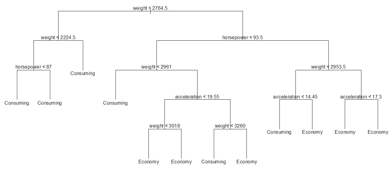
1) root 392 543.400 Consuming ( 0.50000 0.50000 )

2) weight < 2764.5 191 123.700 Economy ( 0.09948 0.90052 )

4) weight < 2224.5 98 11.160 Economy ( 0.01020 0.98980 )

8) horsepower < 87 92 0.000 Economy ( 0.00000 1.00000 ) *

9) horsepower > 87 6 5.407 Economy ( 0.16667 0.83333 ) *

5) weight > 2224.5 93 91.390 Economy ( 0.19355 0.80645 ) *

3) weight > 2764.5 201 147.000 Consuming ( 0.88060 0.11940 )

6) horsepower < 93.5 35 48.260 Consuming ( 0.54286 0.45714 )

12) weight < 2961 8 6.028 Economy ( 0.12500 0.87500 ) *

13) weight > 2961 27 34.370 Consuming ( 0.66667 0.33333 )

26) acceleration < 19.55 17 12.320 Consuming ( 0.88235 0.11765 )

52) weight < 3018 5 6.730 Consuming ( 0.60000 0.40000 ) *

53) weight > 3018 12 0.000 Consuming ( 1.00000 0.00000 ) *

27) acceleration > 19.55 10 12.220 Economy ( 0.30000 0.70000 )

54) weight < 3260 5 0.000 Economy ( 0.00000 1.00000 ) *

55) weight > 3260 5 6.730 Consuming ( 0.60000 0.40000 ) *

7) horsepower > 93.5 166 64.130 Consuming ( 0.95181 0.04819 )

14) weight < 2953.5 21 25.130 Consuming ( 0.71429 0.28571 )

28) acceleration < 14.45 5 5.004 Economy ( 0.20000 0.80000 ) *

29) acceleration > 14.45 16 12.060 Consuming ( 0.87500 0.12500 ) *

15) weight > 2953.5 145 21.110 Consuming ( 0.98621 0.01379 )

30) acceleration < 17.3 128 0.000 Consuming ( 1.00000 0.00000 ) *

31) acceleration > 17.3 17 12.320 Consuming ( 0.88235 0.11765 ) *

Example – the first internal node (the first split). The tree splits all 392 cars in the root into 191 cars with weight < 2764.5 (node 2) and the other 201 cars with weight > 2764.5 (node 3). Among the first group of 191 cars, the deviance is 123.7 (the smaller the better fit). Without any additional data, the tree classifies these cars as “Economy”, the class that makes 90% of this group. The other 201 cars with weight > 2764.5 are classified by the tree as “Consuming”, and in fact, 88% of them are “Consuming”.

Plot. This tree can be visualized.

> plot(tree.fit, type="uniform") # The default type is “proportional”, reflecting the misclassification rate

> text(tree.fit)

> summary(tree.eco)

Number of terminal nodes: 12

Residual mean deviance: 0.3833 = 145.7 / 380

Misclassification error rate: 0.07398 = 29 / 392

This misclassification rate is deceptive, because it is based on the training data.

Cross-validation. Estimate the correct classification rate by cross-validation…

> n = length(ECO); Z = sample(n,n/2);

> tree.eco = tree( ECO ~ horsepower + weight + acceleration, data=Cars[Z,] )

> ECO.predict = predict( tree.eco, Cars, type="class" )

> table( ECO.predict[-Z], ECO[-Z] ) # Confusion matrix

Consuming Economy

Consuming 77 5

Economy 25 89

> mean( ECO.predict[-Z] == ECO[-Z] )

[1] 0.8469388

That’s the classification rate, 84.7% of cars are classified correctly by our tree.

Pruning.

There is built-in cross-validation to determine the optimal complexity of a tree…

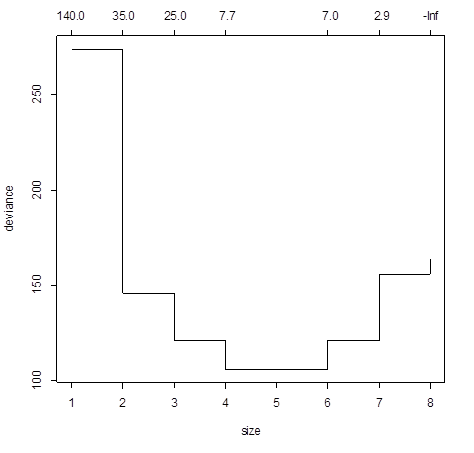
> cv=cv.tree( tree.eco )

> cv

$size # Number of terminal nodes

[1] 8 7 6 4 3 2 1

$dev # Deviance

[1] 163.8182 155.7427 121.3029 106.0917 121.2573 145.9874 273.9971$k

$k # Complexity parameter

[1] -Inf 2.866748 7.045125 7.727424 25.296234 34.517285 137.695468

Deviance is minimized by 4 nodes

> plot(cv)

# Optimize by the smallest mis-classification error instead of deviance…

> cv=cv.tree( tree.eco, FUN = prune.misclass ) # By default (without specified FUN), results are sorted by deviance.

> cv # With “FUN=prune.misclass”, the misclassification rate is the criterion.

$size

[1] 8 7 6 2 1

$dev # Now (despite the name) this is the number of mis-classified units

[1] 26 26 28 25 94 # It is minimized by size=2

> plot(cv)

# We can now prune the tree to the optimal size…

> tree.eco.pruned = prune.misclass( tree.eco, best=2 )

> tree.eco.pruned

1) root 196 271.40 Economy ( 0.47959 0.52041 )

2) weight < 3050.5 114 96.03 Economy ( 0.14912 0.85088 ) *

3) weight > 3050.5 82 37.66 Consuming ( 0.93902 0.06098 ) *

2. Regression trees

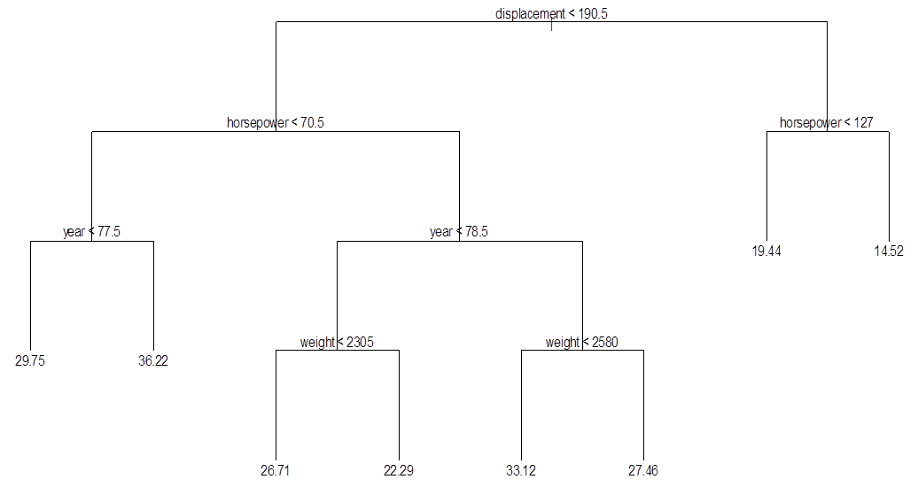
> tree.mpg = tree( mpg ~ .-name-origin+as.factor(origin), Auto )

> tree.mpg

node), split, n, deviance, yval

* denotes terminal node

1) root 392 23820.0 23.45

2) displacement < 190.5 222 7786.0 28.64

4) horsepower < 70.5 71 1804.0 33.67

8) year < 77.5 28 280.2 29.75 *

9) year > 77.5 43 814.5 36.22 *

5) horsepower > 70.5 151 3348.0 26.28

10) year < 78.5 94 1222.0 24.12

20) weight < 2305 39 362.2 26.71 *

21) weight > 2305 55 413.7 22.29 *

11) year > 78.5 57 963.7 29.84

22) weight < 2580 24 294.2 33.12 *

23) weight > 2580 33 225.0 27.46 *

3) displacement > 190.5 170 2210.0 16.66

6) horsepower < 127 74 742.0 19.44 *

7) horsepower > 127 96 457.1 14.52 *

# Now, prediction for each class is the sample mean.

> plot(tree.mpg, type="uniform"); text(tree.mpg)

> summary(tree.mpg)

Regression tree: tree(formula = mpg ~ . - name - origin + as.factor(origin), data = Auto)

Variables actually used in tree construction:

[1] "displacement" "horsepower" "year" "weight"

Number of terminal nodes: 8

Residual mean deviance: 9.346 = 3589 / 384

Distribution of residuals:

Min. 1st Qu. Median Mean 3rd Qu. Max.

-9.4170 -1.5190 -0.2855 0.0000 1.7150 18.5600